It is my blog: where I can share with people all my technical articles about Microsoft techologies and more: AI, AR, Cognitive System, Machine Learning, Robotics, etc.
A lot of interests are visible everywhere how to integrate R scripts with Microsoft PowerBI dashboards. Here goes a step by step guidance on this.
Lets assume, you have some couple of readymade R code available, for example , with ggplot2 library. Lets find the following scripts performing analytics using CHOL data.
Open R studio or R Package (CRAN) & install ggplot2 library first.
Paste the following R script & execute it.
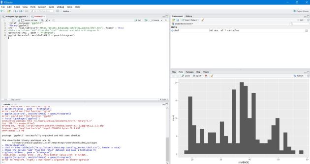
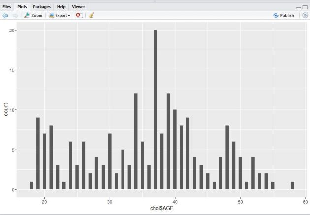
install.packages(‘ggplot2’) library(ggplot2) chol <- read.table(url(“http://assets.datacamp.com/blog_assets/chol.txt”), header = TRUE) #Take the column “AGE” from the “chol” dataset and make a histogram it qplot(chol$AGE , geom = “histogram”) ggplot(data-chol, aes(chol$AGE)) + geom_histogram()
you should be able to see the visuals output like this.
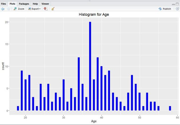
3. Next, execute the following pieces of R code to find out the binwidth argument using ‘qplot()‘ function.
#Lets take help from hist() function qplot(chol$AGE, geom=”histogram”, binwidth = 0.5, main = “Histogram for Age”, xlab = “Age”, fill=I(“blue”))
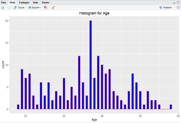
5. Now, add I() function where nested color.
#Add col argument, I() function where nested color. qplot(chol$AGE, geom=”histogram”, binwidth = 0.5, main = “Histogram for Age”, xlab = “Age”, fill=I(“blue”), col=I(“red”))
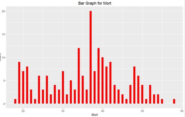
6. Next, adjust ggplot2 little by the following code.
#Plotting Bar Graph qplot(chol$AGE, geom=”bar”, binwidth = 0.5, main = “Bar Graph for Mort”, xlab = “Mort”, fill=I(“Red”))
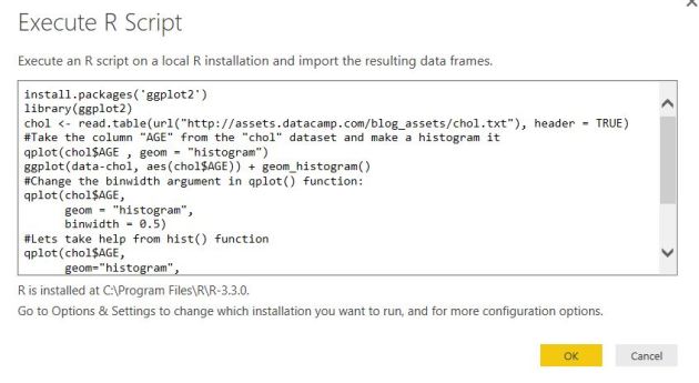
8. Next, open PowerBI desktop tool. You can download it free from this link. Now, click on Get Data tab to start exploring & connect with R dataset.
If you already have R installed in the same system building PowerBI visuals , you just need to paste the R scripts next in the code pen otherwise , you need to install R in the system where you are using the PowerBI desktop like this.
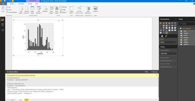
9. Next, you can also choose the ‘custom R visual’ in PowerBI desktop visualizations & provide the required R scripts to build visuals & finally click ‘Run’.
10. Build all the R function visuals by following the same steps & finally save the dashboard.
11.You can refresh an R script in Power BI Desktop. When you refresh an R script, Power BI Desktop runs the R script again in the Power BI Desktop environment.
In the modern IoT Solutions often we have a big number of devices, connected to the back end: thousands hundred thousands or even millions of devices. All these devices should have initial configuration and to be successfully connected to the back-end and this configuration should be done automatically.
In a sequence of article there will be described the main concepts of automatic provisioning and best practices how to implement it (focusing more on Azure based IoT solutions).
Challenges:
If devices are configured in advance during the manufacturing it will be:
1. very difficult to know in advance the connection settings during the manufacturing. For big solutions it is possible to know the customer, but it is difficult to know details about exact connection in advance.
2. Setting the connection in advance is not secure. This approach will give options if somebody know the settings to initiate connection from a fake device and to compromise the system.
3. In the modern IoT solutions it is recommended to have implemented MFA (multi factor authentication).
To be possible to have zero touch provisioning is needed to have pre-set of the devices from the back-end.
This initial configuration includes 2 groups of settings:
Settings, related to the exact connection of the devices to the back-and : end point and authentication
Settings, related to the specific IoT Solution business logic as logical grouping of the devices, which could be done from the back-end
The first group of settings needs communication between back-end and devices to let them know it’s connection and to provide authentication.
How is possible devices to have automated configuration? The most common approach is to have a common “discovery” service for the whole solution. This service will not be changed and devices will connect to this service to receive its settings.
To provide MFA for device registration information on manufactured devices with their specific properties should be imported in advance in the system. This import should be based on the information, provided from the device’s manufacturer. It will be not possible somebody non-authenticated from outside to provide this production data import.
Authentication of devices for initial provision should be provided using 2 independent channels (MFA). Usually those c channels are:
Import of the manufactured device data
Authentication of devices to establish communication channel, used for provisioning
Authentication of devices to establish connection for initial provisioning can be done in several ways:
Basic authentication (not recommended)
Integrated authentication using identity management system like Microsoft Active Directory
Secure attestation using .X.509 or TPM-based identities
Using authentication with specific credentials brings more complexity and more risk. Most of the modern IoT solutions are designed to use secured connection, based on certificates in different varieties.
The both parts of the authentication are 2 sequential parts of the provisioning process.
Manufacturing step.
Solution setup step (back-end setup and device initiated provisioning).
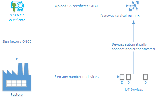
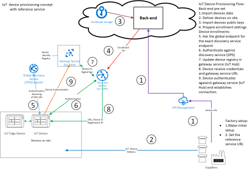
Fig.1 Provisioning based on manufactured devices data and certificates.
Manufacturing step contains:
Base software install and setup.
Configuring pre-requisites for device provisioning: global endpoint, certificate etc.
The back-end setup includes:
Importing information about devices to the back-end system.
Integration with PKI (importing of public certificates in the IoT Solution) – when certificate based security is implemented
Integration with identity management system – when authentication is based on this approach.
Configuring an appropriate discovery service (IoT Hub Device Provisioning Service in Azure), which is able to assist during the provisioning and when device is authenticated to sent the settings to the correct gateway service (IoT Hub).
When the back-end configuration is done it is possible to start the provisioning process, initiated from the device.
Fig.2 describes detailed the common approach for modern zero-touch device provisioning.
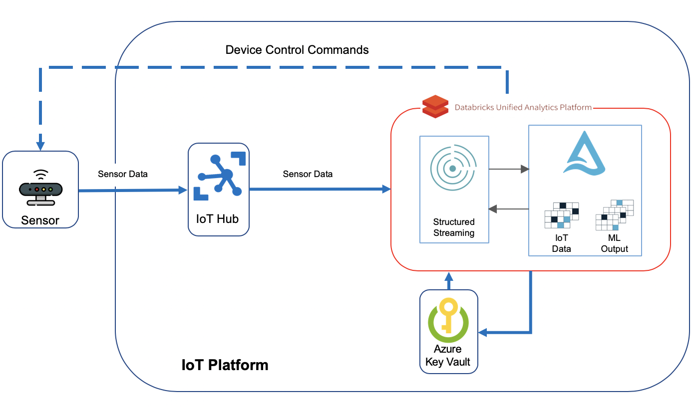
Today I would like to talk about how we can build a serverless solution on Azure that would take us one step closer to powering industrial machines with AI, using the same technology stack that is typically used to deliver IoT analytics use cases. I demoed a solution that received data from an IoT device, in this case a crane, compared the data with the result of a machine learning model that has ran and written its predictions to a repository, in this case a CSV file, and then decided if any actions needs to be taken on the machine, e.g. slowing the crane down if the wind picks up. My solution had 3 main components:
1- IoT Hub: The gateway to cloud, where IoT devices connect and send data to
2- Databricks: The brain of the solution where the data received from IoT device is compared with what the ML algorithm has predicted, and then decided if to take any actions
3- Azure Functions: A Java function was deployed to Azure Functions to call a Direct Method on my simulated crane and instruct it to slow down. Direct Method, or device method, provide the ability to control the behaviour of IoT devices from the cloud.
Since then, I upgraded my solution by moving the part responsible for sending direct methods to IoT devices from Azure Functions into Databricks, as I promised at the end of my talk. Doing this has a few advantages:
The solution will be more efficient since the data received from IoT devices hops one less step before the command is sent back and there are no delays caused by Azure Functions.
The solution will be more simplified, since there are less components deployed in it to get the job done. The less the components and services in a solution, the lower the complexity of managing and running it
The solution will be cheaper. We won’t be paying for Azure Functions calls, which could be pretty considerable amount of money when there are millions of devices connecting to cloud
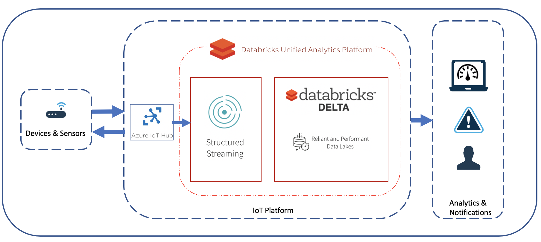
This is what the solution I will go through in this post looks like:
I must mention here that I am not going to store the incoming sensor data as part of this blog post, but I would recommend to do so in Delta tables if you’re looking for a performant and modern storage solution.
Azure IoT Hub
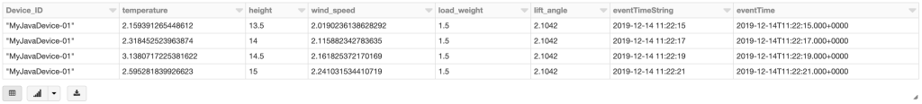
IoT Hub is the gateway to our cloud-based solution. Devices connect to IoT Hub and start sending their data across. I explained what needs to be done to set up IoT Hub and register IoT devices with it in my previous post. I just upgraded “SimulatedDevice.java” to resemble my simulated crane and send additional metrics to cloud: “device_id”, “temperature”,”humidity”,”height”,”device_time”,”latitude”,”longitude”,”wind_speed”,”load_weight” and”lift_angle”. Most of these metrics will be used in my solution in one way or another. A sample record sent by the simulated crane looks like below:
Machine Learning
Those who know me are aware that I’m not a data scientist of any sort. I understand and appreciate most of the machine learning algorithms and the beautiful mathematical formulas behind them, but what I’m more interested in is how we can enable using those models and apply them to our day to day lives to solve problems in form of industry use cases.
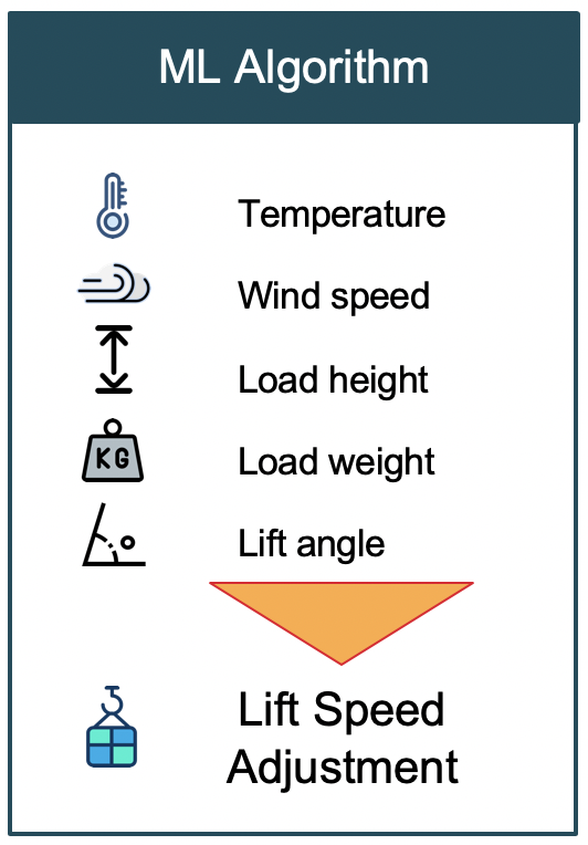
For the purpose of this blog post, I assumed that there was an ML model that has ran and made its predictions on how much the crane needs to slow down based on what is happening in the field in terms of metrics sent by sensors installed on the crane:
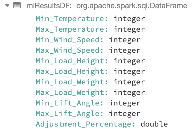
This is how the sample output from our assumed ML model looks like:
As an example to clarify what this output means, let’s look at the first row. It specifies if temperature is between 0 and 10 degrees of celsius, and wind speed is between 0 and 5 km/h, and load height is between 15 and 20 meters, and load weight is between 0 and 2 tons, and load lift angle was between 0 and 5 degrees, then the crane needs to slow down by 5 percent. Let’s see how we can use this result set and take actions on our crane based on the data we receive in real time.
Azure Key Vault
There are a couple of different connection strings that we need for our solution to work, such as “IoT Hub event hub-compatible” and “service policy” connection strings. When building production grade solutions, it’s important to store sensitive information such as connection strings in a secure way. I will show how we can use plain-text connection string as well as accessing one stored in Azure Key Vault in the following sections of this post.
Our solution needs a way of connecting to the IoT Hub to invoke direct methods on IoT devices. For that, we need to get the connection string associated with Service policy of the IoT Hub using the following Azure cli command:
az iot hub show-connection-string --policy-name service --name <IOT_HUB_NAME> --output table
And store it in Azure Key Vault. So go ahead and create an Azure Key Vault and then:
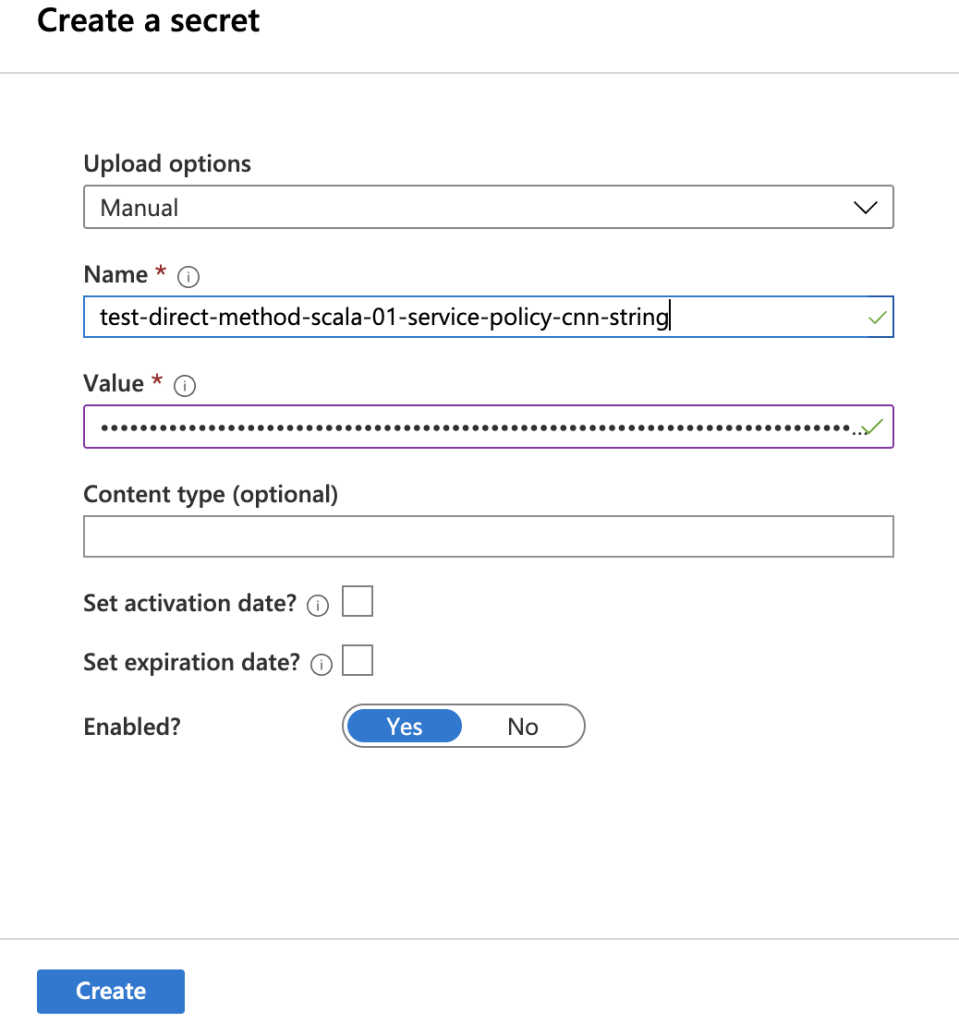
Click on Secrets on the left pane and then click on Generate/Import
Select Manual for Upload options
Specify a Name such as <IOT_HUB_NAME>-service-policy-cnn-string
Paste the value you got from the above Azure Cli command in the Value text box
After completing the steps above and creating the secret, we will be able to use the service connection string associated with the IoT Hub in the next stages of our solution, which will be built in Databricks.
Databricks
In my opinion, the second most important factor separating Artificial Intelligence from other kinds of intelligent systems, after the complexity and type of algorithms, is the ability to process data and respond to events in real time. If the aim of AI is to replace most of human’s functionalities, the AI-powered systems must be able to mimic and replicate human brain’s ability to scan and act as events happen.
I am going to use Spark Streaming as the mechanism to process data in real time in this solution. The very first step is to set up Databricks, you can read on how to do that in my previous blog post. Don’t forget to install “azure-eventhubs-spark_2.11:2.3.6” library as instructed there. The code snippets you will see in the rest of this post are in Scala.
Load ML Model results
To be able to use the the results of our ML model, we need to load it as a Dataframe. I have the file containing the sample output saved in Azure Blob Storage. What I’ll do first is to mount that blob in DBFS:
To get Storage_Account_Key, navigate to your storage account in Azure portal, click on Access Keys from left pane and copy the string under Key1 -> Key.
After completing above steps, we will be able to use the mount point in the rest of our notebook, which is much easier than having to refer to the storage blob every time. The next code snippet shows how we can create a Dataframe using the mount point we just created:
val CSV_FILE="/mnt/ml-output/ml_results.csv"
val mlResultsDF = sqlContext.read.format("csv")
.option("header","true")
.option("inferSchema","true")
.load(CSV_FILE)
Executing the cell above in Databricks notebook creates a DataFrame containing the fields in the sample output file:
Connect to IoT Hub and read the stream
This step is explained in my previous blog post as well, make sure you follow the steps in “Connect to IoT Hub and read the stream” section. For the reference, Below is the Scala code you would need to have in the next cell in the Databricks notebook:
import org.apache.spark.eventhubs._
import org.apache.spark.eventhubs.{ ConnectionStringBuilder, EventHubsConf, EventPosition }
import org.apache.spark.sql.functions.{ explode, split }
val connectionString = ConnectionStringBuilder("<Event hub connection string from Azure portal>").setEventHubName("<Event Hub-Compatible Name>")
.build
val eventHubsConf = EventHubsConf(connectionString)
.setStartingPosition(EventPosition.fromEndOfStream)
.setConsumerGroup("<Consumer Group>")
val sensorDataStream = spark.readStream
.format("eventhubs")
.options(eventHubsConf.toMap)
.load()
Apply structure to incoming data
Finishing previous step gives us a DataFrame containing the data we receive from our connected crane. If we run a display command on the DataFrame, we see that the data we received does not really resemble what is sent by the simulator code. That’s because the data sent by our code actually goes into the first column, body, in binary format. We need to apply appropriate schema on top of that column to be able to work with the incoming data with structured mechanism, e.g. SQL.
Defines the schema matching the data we produce at source
Applies the schema on the incoming binary data
Extracts the fields in a structured format including the time the record was generated at source, eventTime
Uses the eventTime column to define watermarking to deal with late arriving records and drop data older than 5 seconds
The last point is important to notice. The solution we’re building here is to deal with changes in the environment where the crane is operating in, in real-time. This means that the solution should wait for the data sent by the crane only for a limited time, in this case 5 seconds. The idea is that the solution shouldn’t take actions based on old data, since a lot may change in the environment in 5 seconds. Therefore, it drops late records and will not consider them. Remember to change that based on the use case you’re working on.
Running display on the resulting DataFrame we get following:
display(sensorDataDF)
Decide when to take action
Now that we have both the ML model results and IoT Device data in separate DataFrames, we are ready to code the logic that defines when our solution should send a command back to the device and command it to slow down. One point that is worth noticing here is that the mlResultsDF is a static DataFrame whereas sensorDataDF is a streaming one. You can check that by running:
println(sensorDataDF.isStreaming)
Let’s go through what needs to be done at this stage one more time: as the data streams in from the crane, we need to compare it with the result of the ML model and slow it down when the incoming data falls in the range defined by the ML model. This is easy to code: all we need to do is to join the 2 datasets and check for when this rule is met:
The result of running above cell in Databricks notebook would be a streaming DataFrame which contains the records our solution need to act upon.
Connect to IoT Hub where devices send data to
Now that we have worked out when our solution should react to incoming data, we can move to the next interesting part which is defining how and what of taking action on the device. We already discussed that an action is taken on the crane by calling a direct method. This method instructs crane to slow down by the percentage that is passed in as the parameter. If you look into the SimulatedDevice.java file in the azure-iot-samples-java github repo, there is a switch expression in the “call” function of “DirectMethodCallback” class which defines the code to be executed based on the different direct methods called on the IoT device. I extended that to simulate crane being slowed down, but you can work with the existing “SetTelemetryInterval” method.
So, what we need to do at this stage is to connect to the IoT Hub where the device is registered with from Databricks notebook, and then invoke the direct method URL which should be in the form of “https://{iot hub}/twins/{device id}/methods/?api-version=2018-06-30“
To authenticate with IoT Hub, we need to create a SAS token in form of “SharedAccessSignature sig=<signature>&se=<expiryTime>&sr=<resourceURI>”. Remember the service level policy connection string we put in Azure Key Vault? We are going to use that to build the SAS Token. But first, we need to extract the secrets stored in Key Vault:
val vaultScope = "kv-scope-01"
var keys = dbutils.secrets.list(vaultScope)
val keysAndSecrets = collection.mutable.Map[String, String]()
for (x <- keys){
   val scopeKey = x.toString().substring(x.toString().indexOf("(")+1,x.toString().indexOf(")"))
   keysAndSecrets += (scopeKey -> dbutils.secrets.get(scope = vaultScope, key = scopeKey) )
}
After running the code in above cell in Databricks notebook, we get a map of all the secrets stored in the Key Vault in form of (“Secret_Name” -> “Secret_Value”).
Next, we need a function to build the SAS token that will be accepted by IoT Hub when authenticating the requests. This function will do the followings:
Uses the IoT Hub name to get the service policy connection string from the Map of secrets we built previously
Extracts components of the retrieved connection string to build host name, resource uri and shared access key
Computes a Hash-based Message Authentication Code (HMAC) by using the SHA256 hash function, from the shared access key in the connection string
Uses an implementation of “Message Authentication Code” (MAC) algorithm to create the signature for the SAS Token
And finally returns SharedAccessSignature
import javax.crypto.Mac
import javax.crypto.spec.SecretKeySpec
import java.net.URLEncoder
import java.nio.charset.StandardCharsets
import java.lang.System.currentTimeMillis
val iotHubName = "test-direct-method-scala-01"
object SASToken{
   def tokenBuilder(deviceName: String):String = {
        val iotHubConnectionString = keysAndSecrets(iotHubName+"-service-policy-cnn-string")
        val hostName = iotHubConnectionString.substring(0,iotHubConnectionString.indexOf(";"))
        val resourceUri = hostName.substring(hostName.indexOf("=")+1,hostName.length)
        val targetUri = URLEncoder.encode(resourceUri, String.valueOf(StandardCharsets.UTF_8))
        val SharedAccessKey = iotHubConnectionString.substring(iotHubConnectionString.indexOf("SharedAccessKey=")+16,iotHubConnectionString.length)//iotHubConnectionStringComponents(2).split("=")
        val currentTime = currentTimeMillis()
        val expiresOnTime = (currentTime + (365*60*60*1000))/1000
        val toSign = targetUri + "\n" + expiresOnTime;
        var keyBytes = java.util.Base64.getDecoder.decode(SharedAccessKey.getBytes("UTF-8"))
        val signingKey = new SecretKeySpec(keyBytes, "HmacSHA256")
        val mac = Mac.getInstance("HmacSHA256")
        mac.init(signingKey)
        val rawHmac = mac.doFinal(toSign.getBytes("UTF-8"))
        val signature = URLEncoder.encode(
        new String(java.util.Base64.getEncoder.encode(rawHmac), "UTF-8"))
        val sharedAccessSignature = s"Authorization: SharedAccessSignature sr=test-direct-method-scala-01.azure-devices.net&sig="+signature+"&se="+expiresOnTime+"&skn=service"
        return sharedAccessSignature
   }
}
The code above is the part I am most proud of getting to work as part of this blog post. I had to go through literally several thousands of lines of Java code to figure out how Microsoft does it, and convert it to Scala. But please let me know if you can think of a better way of doing it.
Take action by invoking direct method on the device
All the work we did so far was to prepare for this moment: to be able to call a direct method on our simulated crane and slow it down based on what the ML algorithm dictates. And we need to be able to do so as records stream into our final DataFrame, joinedDF. Let’s define how we can do that.
We need to write a class that extends ForeachWrite. This class needs to implement 3 methods:
open: used when we need to open new connections, for example to a data store to write records to
process: the work to be done whenever a new record is added to the streaming DataFrame is added here
close: used to close the connection opened in first method, if any
We don’t need to open and therefore close any connections, so let’s check the process method line by line:
Extracts device name from incoming data. If you run a display on joinedDF, you’ll see that the very first column is the device name
Builds “sharedAccessSignature” bu calling SASToken.tokenBuilder and passing in the device name
Builds “deviceDirectMethodUri” in ‘{iot hub}/twins/{device id}/methods/’ format
Builds “cmdParams” to include the name of the method to be called, response timeout, and the payload. Payload is the adjustment percentage that will be sent to the crane
Builds a curl command with the required parameters and SAS token
The very last step is to call the methods we defined in the StreamProcessor class above as the records stream in from our connected crane. This is done by calling foreach sink on writeStream:
val query =
   joinedDF
      .writeStream
      .foreach(new StreamProcessor())
      .start()
And we’re done. We have solution that is able to control theoretically millions of IoT devices using only 3 services on Azure.
The next step to go from here would be to add security measures and mechanisms to our solution, as well as monitoring and alerting. Hopefully I’ll get time to do them soon.
IoT devices produce a lot of data very fast. Capturing data from all those devices, which could be at millions, and managing them is the very first step in building a successful and effective IoT platform.
Like any other data solution, an IoT data platform could be built on-premise or on cloud. I’m a huge fan of cloud based solutions specially PaaS offerings. After doing a little bit of research I decided to go with Azure since it has the most comprehensive and easy to use set of service offerings when it comes to IoT and they are reasonably priced. In this post, I am going to show how to build the architecture displayed in the diagram below: connect your devices to Azure IoT Hub and then ingest records into Databricks Delta Lake as they stream in using Spark Streaming.
Solution Architecture
Setup Azure IoT Hub and Register a Device
The very first step is to set up Azure IoT Hub, register a device with it and test it by sending data across. This is very well explained by Microsoft here. Make sure you follow all the steps and you’re able to read the messages sent to IoT Hub at the end.
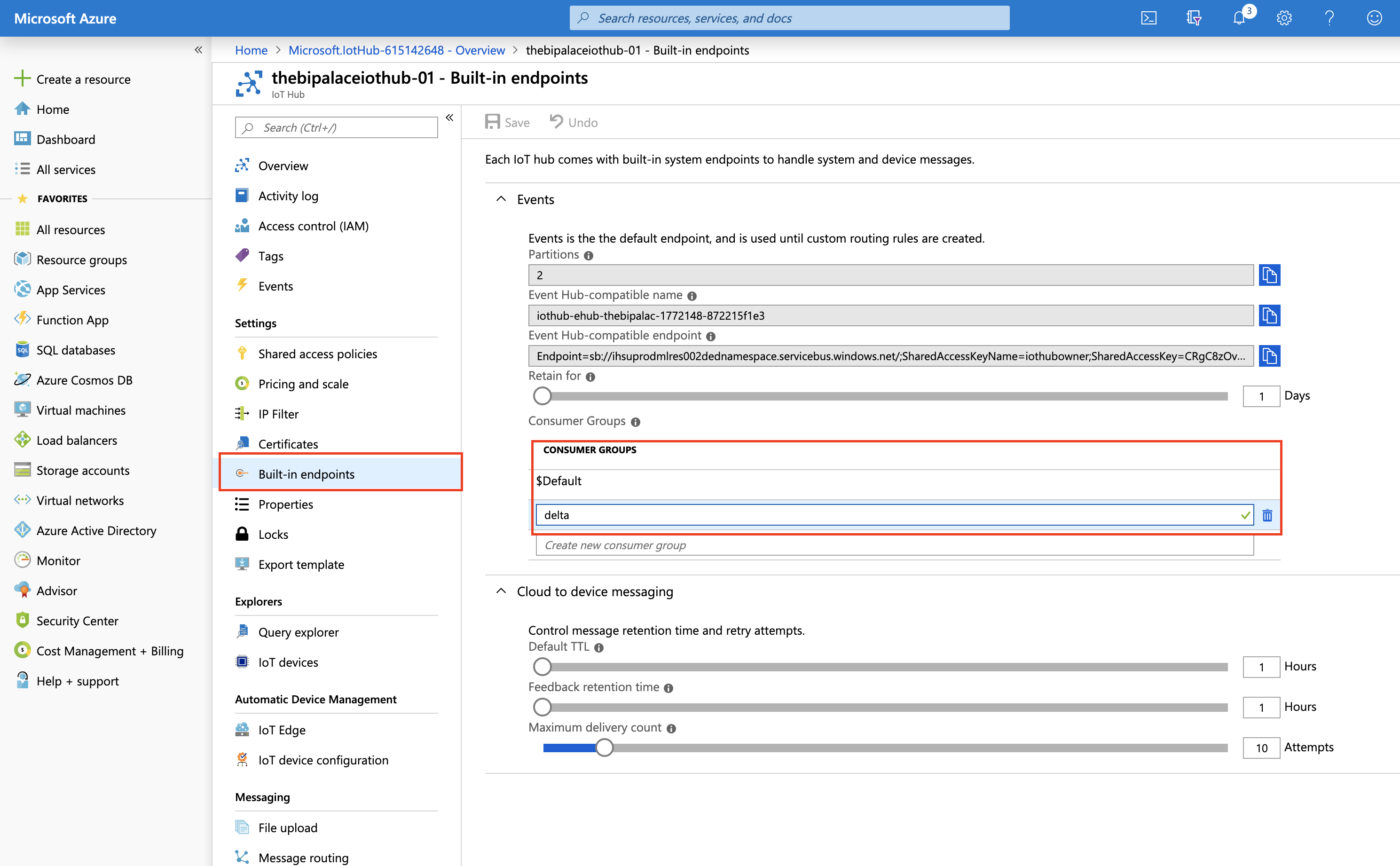
The only extra step we need to take is to add a new consumer group to the IoT Hub. Doing this means our Spark Streaming application will have its own offset, tracking where in the queue it has last read the records coming from devices. By assigning unique consumer groups to each application that subscribes to IoT Hub, we can send the record coming from IoT devices to multiple destinations, for example to store them in Blob storage, send them to Azure Stream Analytics and do real-time analytics, as well as a delta table in Databricks Delta Lake.
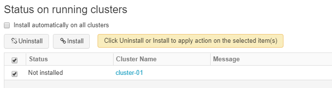
Navigate to IoT Hub page on the Azure portal and select your hub. Click on Built-in endpoints and add a new Consumer Group:
Add Consumer Group to IoT Hub
Databricks: Unified Analytics Platform & Delta Lake
Moving on to the next layer in our architecture, we’re going to set up Databricks. Databricks offers a platform that unifies data engineering, data science and business logic. It is basically PaaS offering for Spark on cloud, which speeds up data exploration and preparation.
Why Delta?
Delta Lake is a storage layer invented by Databricks to bring ACID transactions to big data workloads. This is a response to limitation within the existing big data storage mechanisms like Parquet: They are immutable. To update a record within a Parquet file, you need to re-write the whole file. With Delta, you can easily write update statements at records level. This is all we need to know about Delta file format for the purpose of what we want to build here, more about is here.
A very important result of this feature for IoT and streaming use cases is that we will be able to query the data as they arrive, instead of having to wait for a partition to be updated (re-written)
In this solution we will see how to set up Databricks, use Spark Streaming to subscribe to records coming in to Azure IoT Hub, and write them to a Delta table.
Setup Databricks
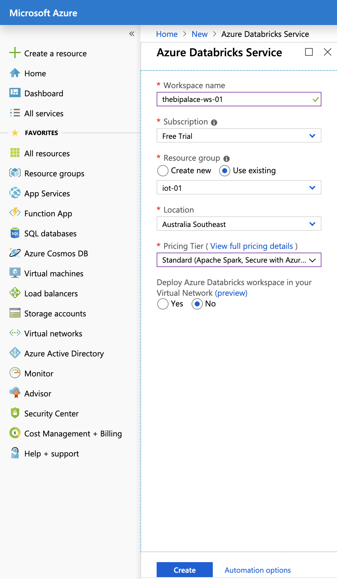
Navigate to Azure Portal and click on Create a Resource -> Analytics -> Azure Databricks. This is where you create a workspace, which is where you can access all your databricks assets. Fill up the new form that opens up and make sure you select Standard for pricing tier. Then hit Create:
Create Databricks Workspace
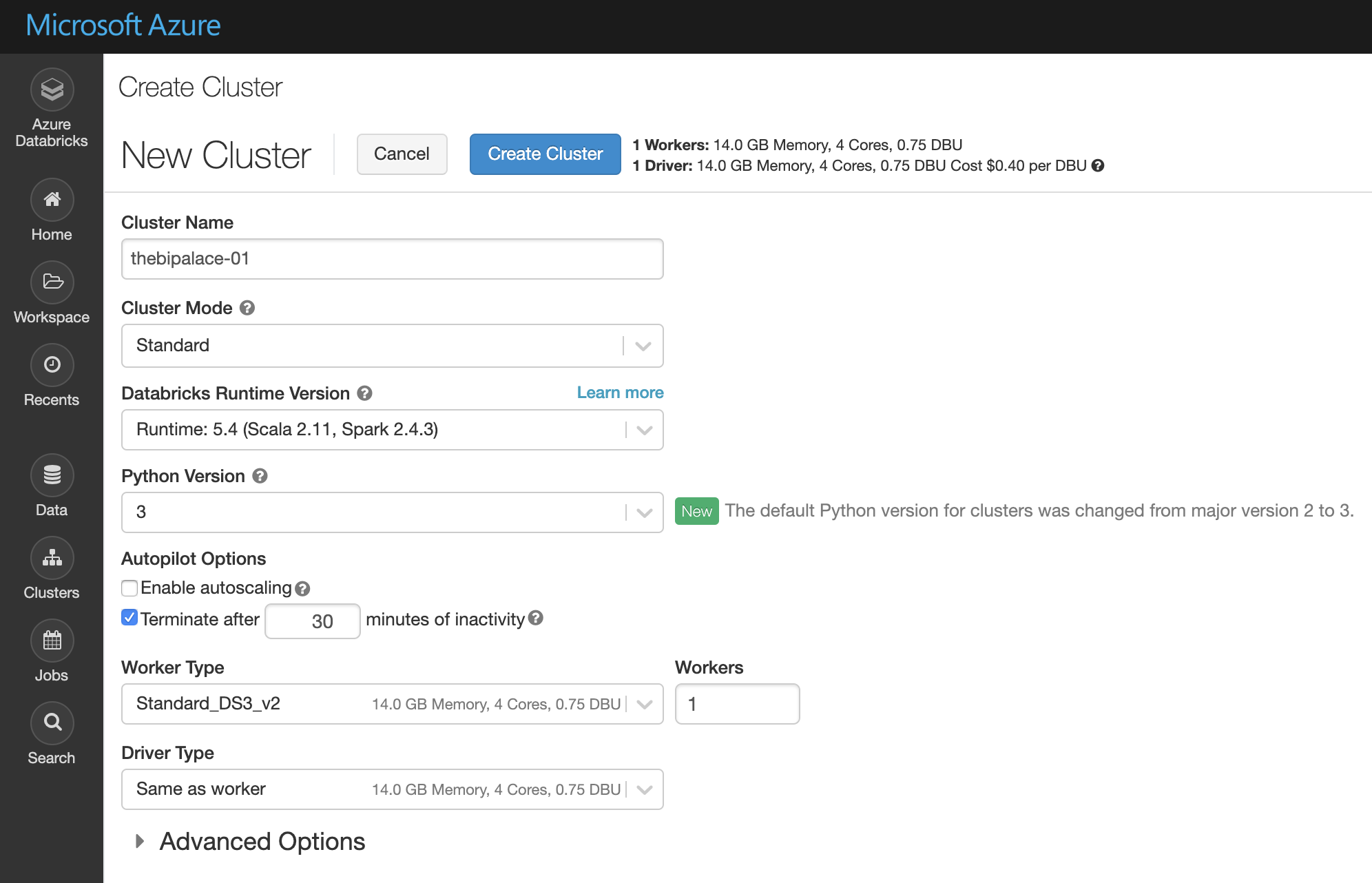
When the workspace is created, go to Azure Databricks Workspace resource page and click on Lunch Workspace. You will be navigated to your workspace. Create a new cluster with the same properties you see in the picture below. You can ask for bigger nodes or enable autoscaling, but it’s not needed for this tutorial:
Create Databricks Cluster
The next step is to create a notebook. Click on Home -> <Your Email Address> -> Create -> Notebook. Give it a name, select Scala as the default language of the notebook (you can change it later using %), and select the cluster where this notebook’s commands will run on.
Structured Streaming from IoT Hub
Create and install required Maven library
For our streaming solution to work, we need to install ” azure-eventhubs-spark_2.11:2.3.6″ Maven library. The steps to do that are very easy:
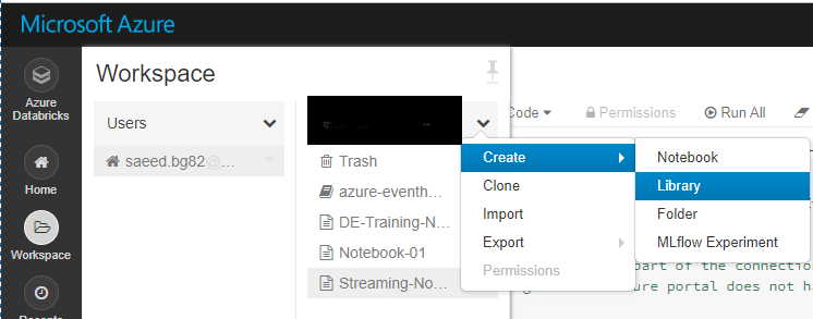
Open the notebook and click on Workspace -> [User_Name] -> Create -> Library:
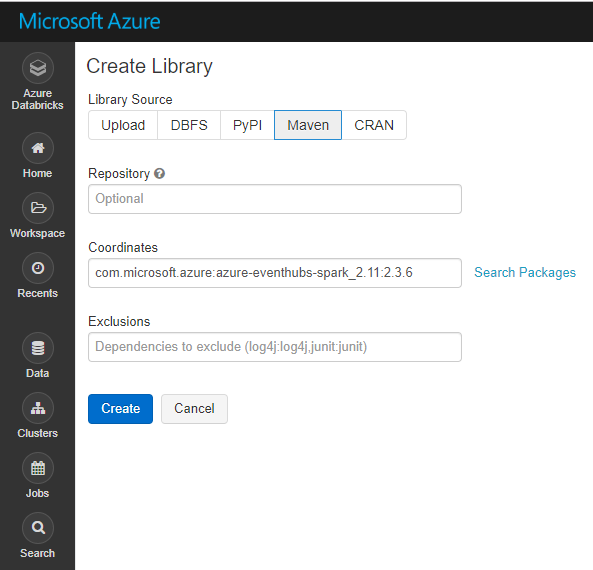
Select Maven and copy and paste ” com.microsoft.azure:azure-eventhubs-spark_2.11:2.3.6″ into Coordinates box, then click on Create:
After the library is created, you’ll be redirected to the page where you can install your library on the existing clusters. Select the cluster where you’ll be running your Spark streaming code and click Install:
Important: You should restart your cluster after the installation is complete for it to take effect.
Connect to IoT Hub and read the stream
import org.apache.spark.eventhubs._
import  org.apache.spark.eventhubs.{ ConnectionStringBuilder, EventHubsConf, EventPosition }
import  org.apache.spark.sql.functions.{ explode, split }

// To connect to an Event Hub, EntityPath is required as part of the connection string.
// Here, we assume that the connection string from the Azure portal does not have the EntityPath part.
val connectionString = ConnectionStringBuilder("--IOT HUB CONNECTION STRING FROM AZURE PORTAL--")
  .setEventHubName("--IoT Hub Name--")
  .build
val eventHubsConf = EventHubsConf(connectionString)
  .setStartingPosition(EventPosition.fromEndOfStream)
  .setConsumerGroup("delta")

val eventhubs = spark.readStream
  .format("eventhubs")
  .options(eventHubsConf.toMap)
  .load()
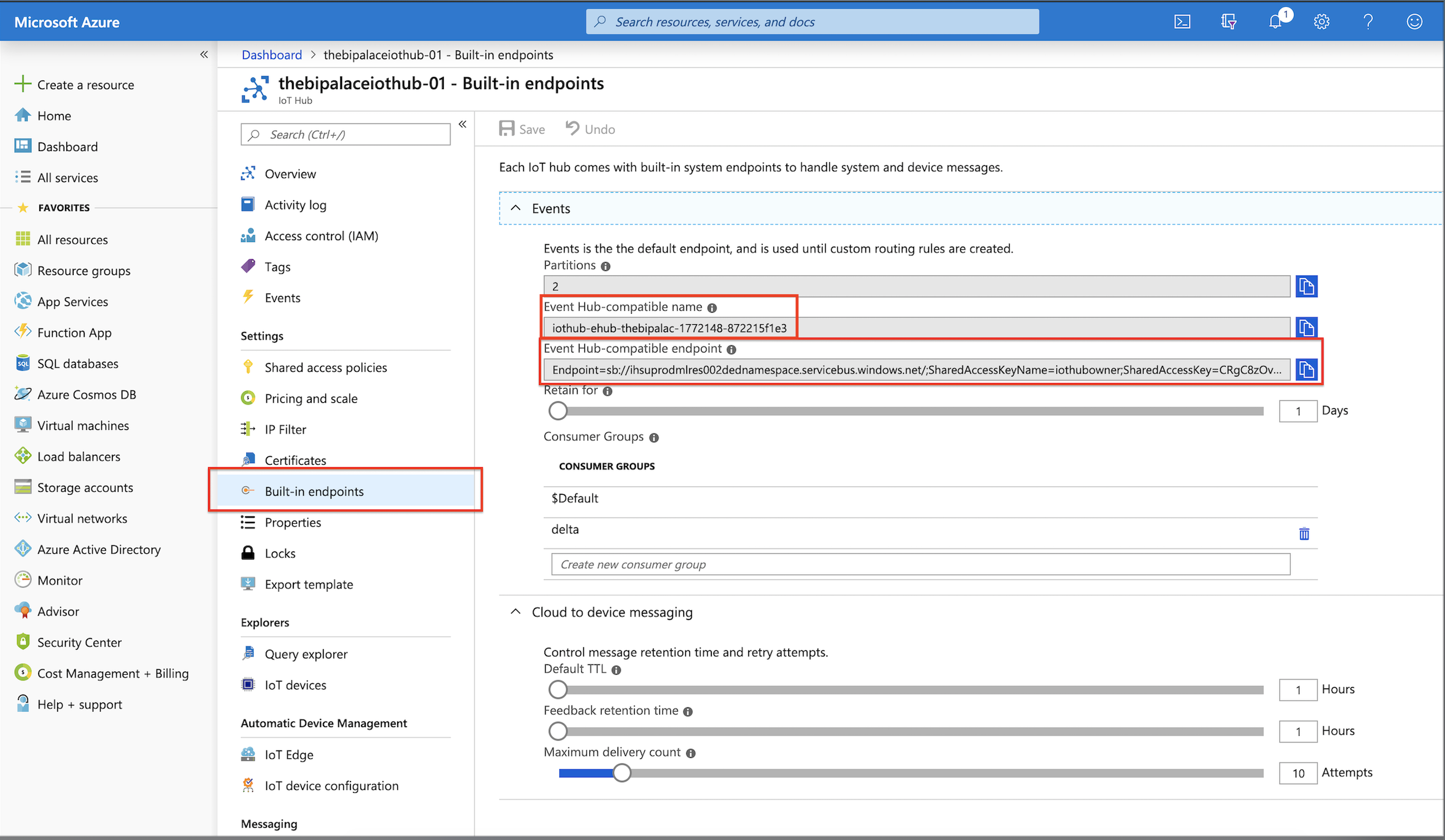
The code snippet above first builds a connection string pointing to the IoT Hub we created before. The only extra steps you need to take is to get the connection string from Azure portal and replace it in ConnectionStringBuilder and then change the name in .setEventHubName to “<Event Hub-compatible name>” accordingly. Open Azure portal and go to your IoT Hub’s page. Click on Built-in endpoints and copy what you see below and paste in the code snippet in the notebook:
IoT Hub Endpoint Details
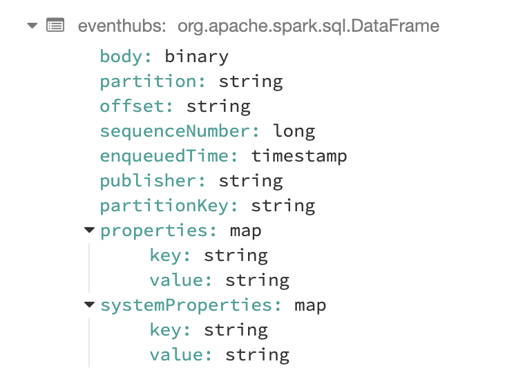
What we get after those commands are completed successfully is a DataFrame that has the following fields in it. The messages coming from our IoT device are in the “body” field:
To see how the incoming data from the IoT sensor looks like just run:
display(eventhubs)
Extract device data and create a Spark SQL Table
The next step would be to extract the device data coming in the body field of the DataFrame we built in previous step and build the DataFrame comprising of the fields we want to store in our Delta Lake to do analytics on later:
import org.apache.spark.sql.types._
import org.apache.spark.sql.functions._
val schema = (new StructType)
    .add("temperature", DoubleType)
    .add("humidity", DoubleType)
val df = eventhubs.select(($"enqueuedTime").as("Enqueued_Time"),($"systemProperties.iothub-connection-device-id")
                  .as("Device_ID"),(from_json($"body".cast("string"), schema)
                  .as("telemetry_json"))).select("Enqueued_Time","Device_ID", "telemetry_json.*")
The resulting DataFrame looks like:
Now we can create a table from our DataFrame and start writing SQL commands on it:
Create the final DataFrame and write stream to Delta table
We’re almost there. We have the data we receive from our IoT device in a Spark SQL table, which enables us to transform it easily with SQL commands.
Tables in a Big Data ecosystem are supposed to be partitioned. I mean they better be, otherwise they’ll cause all sorts of problems. The reason I extracted Enqueued_Time from JSON was to be able to partition my table by date/hour. IoT devices produce a lot of data and partitioning them by hour not only makes each partition reasonably sized, but also enable a certain type of analytics to be performed on the data when companies need to predict the performance of their devices at different times of the day or night, for example.
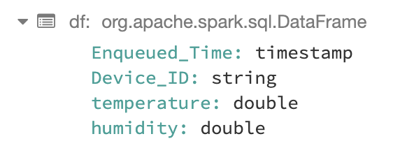
val finalDF = spark.sql("Select Date(Enqueued_Time) Date_Enqueued
, Hour(Enqueued_Time) Hour_Enqueued, Enqueued_Time, Device_ID
, temperature AS Temperature, humidity as Humidity
from device_telemetry_data")
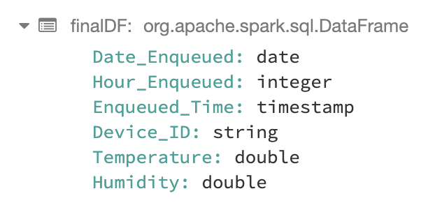
The resulting DataFrame has the following schema:
The final step is to write the stream to a Delta table:
outputMode: Specifies how the records of a streaming DataFrame are written to the streaming sink. There are 2 modes:
Append: Only the new records will be written to the sink
Complete: All records will be written to the sink every time there is an update
Update: Only the updated records will be outputed to sink
option: checkpointLocation
This is needed to ensure fault-tolerance. Basically we specify a location to save all application progress information. This is specially important in case of a Driver failure, read more here.
format: The output sink where the result will be written, obviously “delta”.
partitionBy: The column(s) by which we want our table to be partitioned by. We decided to partition our table hourly as explained above, so we pass in date and hour.
table: The name of the table.
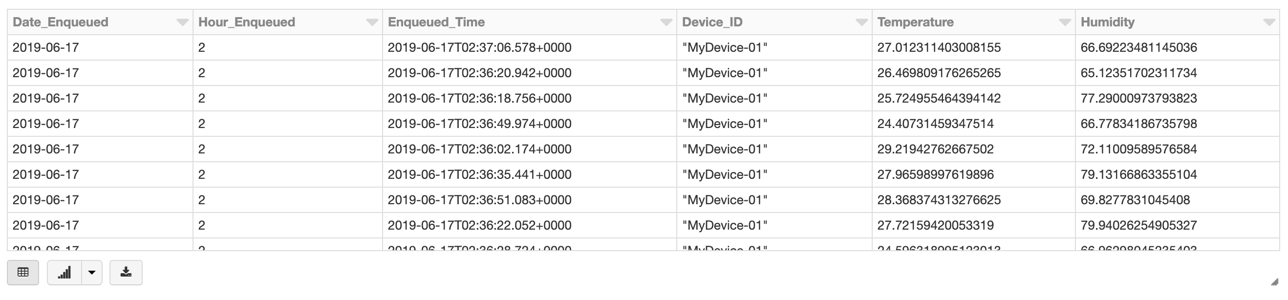
If all the steps above have worked, you should be able to query your table and see the records inserted into the Delta table by running the following command:
%sql
SELECT * FROM delta_telemetry_data
And we’re done! Now we have a table in our Delta Lake that holds our IoT devices data. You can take it from here and do ML on the data collected or mix it with other tables you might have in your Delta Lake. And definitely feel free to ask your questions below in comments section.
I’ve been working on a project and been using CosmosDB as a data source and extracting the data from it into Azure Databricks. Once there I apply some data and analytics magic to it. So this post is about some of the assumptions that I had about it, and some of the issues that I came across.
For setting up Databricks to get data from CosmosDB, the place to go is the Azure CosmosDB Spark connector site. I’m not going to go through installing it, as the read me and guidance on the GitHub does a good job and it is straight forward to do. There is also a tutorial here, that deals with ‘On time flight performance’, it covers how to connect, and then process data but doesn’t cover any of the issues you may have, as its using a nice, conformed data structure. In the real world, we have all sorts of weird design options, taken over the life time of a product and/or service.
I’m using the Databricks Python API to connect to CosmosDB, so the start of setting up a connection is set out here:
Just add your keys etc, everything is nice and straight forward so far. I’ve left out the custom query option for the time being, but I’ll be coming back to it in a bit. The next bit sets up the read format by using the configuration used above, the creates a temp view called in this case “c”.
12345
# Sets up the CosmosDB connection.# Creates a temp table call c, which is used in the query# to define the collectioncosmosdbConnection =spark.read.format("com.microsoft.azure.cosmosdb.spark").options(**cosmosConfig).load()cosmosdbConnection.createOrReplaceTempView("c")
SQL Queries
So now we have created a temp view in Databricks called “c” that sits over CosmosDB, we can create a data frame based on a spark SQL context query. So lets send a Cosmos SQL API style query from Databricks, for example:
12
family = spark.sql(SELECT{"Name":c.id, "City":c.address.city} ASFamilyFROMc WHEREc.address.city = c.address.state)
It should return a error. Why? This was my first mistake, you can’t use the Cosmos SQL API syntax. It will not return a document, but columns and rows like a standard SQL table.
12
family = spark.sql(SELECTc.id ASName, c.city ASCity FROMcWHEREc.city = c.state)
The above will work, but it will return a table like object, not a document like the CosmosDB SQL query.
Tip 1: You can’t use your Cosmos DB SQL queries, they will have to be redone in a more standard SQL syntax, but that is good, we can finally use a “Group by” to query data on CosmosDB!
CosmosDB Document Considerations
One of the issues I came across, was that we have a number of documents in our Cosmos DB, that are split by types, using an “entity” field, so we have for example, Customer and Project documents.
Now if you have the same field name in the documents, but different data types it can get mixed up? How, using this example for “customer”
1234
{ #some other customer JSON here"range":"PWAQ-100","entity":"customer"}
This removes the ” and changes the “:” to “=” rather than a column that contains the array which I can then explode the JSON into other objects. So I get a string back…Weird! Well what happened? Well it’s all down in part to the configuration we set up earlier:
1
"schema_samplesize": "2000"
The first 2000 documents it read to determine the “c” table schema were of the “customer” type and set it as a string. In fact if you do the following query:
1
test_df =spark.sql(SELECT *FROM c)
It will show all the columns for the Customer and Project as one big table, with all repeated columns names and datatypes that have been adjusted to fit the data frames expected schema.
There are three ways to solve this.
Don’t mix datatypes for fields that have same name in your document schema
Don’t store a mixture of document schemas in your CosmosDB database
Use the custom query option
Using Custom Query
If like me you can’t do 1 or 2, you have to use the custom query option. Lets go back to our set up of the connection:
123456789101112
cosmosConfig ={"Endpoint": "https://cloudsuite-test.documents.azure.com:443/","Masterkey": "wxElqnT67i3Ey7Mmh7rH2Opxxwjbn22g6RL8LFjboDK6Cqg6M8COfVcQXaJO3pxLq0vEDayidnisn5QmbN5dPQ==","Database": "cbi_survey","preferredRegions": "UK South","Collection": "cbi","ConnectionMode": "DirectHttps","SamplingRatio": "1.0","schema_samplesize": "20000","query_pagesize": "2147483647","query_custom": "SELECT c.* FROM c WHERE c.entity = 'project'"}
So we have now added the following line to the config:
“query_custom” : “SELECT c.* FROM c WHERE c.entity = ‘project’”
So we now know that we will only get documents back of the schema “project” and should map the datatypes correctly.
12345
# Sets up the CosmosDB connection.# Creates a temp table call c, which is used in the query# to define the collectioncosmosdbConnection =spark.read.format("com.microsoft.azure.cosmosdb.spark").options(**cosmosConfig).load()cosmosdbConnection.createOrReplaceTempView("project")
I’ve also now create a distinct temp view called ‘project’ that I can query. I will do the same for ‘customer’ and any other document schemas stored in Cosmos DB.
Tip 2: Make sure to declare your temp views based on the documents you need
With CosmosDB and Databricks when you create the connection and query, it is schema on read. So it you have added items to your JSON structure, make sure that you set your schema sample size to allow it to read enough items, otherwise a column(s) that is in later version of your document schema, may not read correctly and any SQL queries will fail when you reference that column.
Tip 3: “schema_samplesize” should be adjusted were needed
Now I’ve wrapped up the connection and table details into a function that I can call with my entity value, and it will set that temp view up nice and cleanly.
Overall the Azure Spark Connector is works well and pulling data from Cosmos is fast. Databricks and JSON is a lot easier to handle than querying it in SQL Server, and we have been using it more for some projects for our ETL pipelines.
On the down side, the GitHub site needs a little bit of an update as it has a number of broken links, and a number of open issues that haven’t been looked at or assigned.
Today we are going to start using cognitive services to enhance our solution. We will start simple with just one cognitive service this week, and more over time, including a second one next week. First, we are starting with Bing Image search. The problem? Our sets don’t have a picture of the completed set, and there doesn’t seem to be a downloadable collection of these for us to use. For example, take the Han Solo set below, all we can see is the name, year, total pages, theme, and all of the individual parts.
The solution? We will take the model number, perform a Bing image search, load that image into a storage blob, and add a reference to this image in our database (to optimize the service calls to Bing image search).
Creating the cognitive services item in Azure
First, we will add a cognitive services resource in Azure. Searching for “cognitive services”, we create the new resource, name it, assign it to a resource group, and select the S0 pricing tier.
Pricing is pretty reasonable, especially at this scale, (we only have 5 products), with 1,000 API calls costing only a $1. We are only going to update images for models we are using, rather than populating the entire database (although we may do that later).
In the new Cognitive Services resource, we browse to the “keys” section, and make a note of the subscription key, which we will need in our code shortly.
We also make a note of the cognitive services base url for our region – we deployed this cognitive service in East US:
Now we call the bing api, using the subscription key, our base url, and some parameters to search (“q”), and using the “safesearch” parameter to ensure we only return “safe” results. The rest of the function needs some processing to return the search results.
We call our function, and process the result, getting a image url to the new image. We download this image, save it to a new container in our storage account, and then save the name of the image in a new “set_images” database table, so that we don’t have to do searches over and over.
We incorporate this code into our web service. Now when the web page loads, it checks if the image is in the database. If it finds the image, we display it, if we can’t find one, the service searches Bing, downloads the image to our storage, and then displays a new image. The result for Han Solo is shown below:
It looks pretty good… except for some of the models, it displays a false positive. The picture below is clearly not a “Star Destroyer”…
Creating a page to resolve false positives
To correct this, we create a new web page that displays the first 10 images returned from Bing search, allowing us to select the image we think is best. In this case, the second image is exactly what we are looking for, so we can select that, triggering our application to download this image to our storage account and database.
Wrapup
Our set page now looks great. We’ve used a simple cognitive service to automate a boring manual search process.
There is still more we can do, next week we are going to apply a second layer of cognitive services to only display and select images that contain Lego.
If you want to nail your WordPress site’s SEO and make your website more accessible to visitors with screen readers, you should be adding alt text to all of the images that you use in your content.
However, adding alt text is also time-consuming, especially if you use a lot of images. That makes it easy to forget (or just skip, if you’re feeling lazy).
So what if there were a better way? A way to automatically add accurate, contextual image alt text to your WordPress images using the power of machine learning and artificial intelligence (AI)?
As you can probably guess, there is a better way, and I’m going to show you how to set it up using a free plugin in this post.
How AI-Powered Automatic Image Alt Text Works
The automatic image alt text method that I’m going to show you is based on Microsoft’s Cognitive Services AI, which is part of the Microsoft Azure suite of services. That sounds intimidating, but it’s pretty painless to set up.
Essentially, Microsoft’s Cognitive Services AI can look at an image and then describe what’s happening in plain English.
For example, if you feed it an image of a sheep standing in a grassy field, it can say that the image contains a sheep grazing in a grassy field.
Here’s a real example of what it’s like after setting everything up.
I can upload this image to my WordPress site:
Then, the plugin will hook into Microsoft’s Cognitive Services AI to automatically generate this image alt text without me lifting a finger:
A horse grazing on a lush green field
It even calls the field “lush”. Cool, right?
If you upload a lot of “real” images like the example, this is an awesome way to save some time.
However, this method isn’t perfect, and it won’t work for all types of images.
For example, if you’re uploading detailed interface screenshots (like the images in the rest of this post), the alt text that the tool generates isn’t very accurate because it can’t grasp the detail of what you’re doing in the interface.
I tried uploading one of the screenshots from the tutorial below, and the automatic image alt text wasn’t relevant or useful.
Still, for a lot of WordPress sites, this is a great way to save some time while boosting your SEO and website accessibility.
How to Set Up Automatic Image Alt Text on WordPress
To start using automatic image alt text, you can use the free Automatic Alternative Text plugin from Jacob Peattie.
The plugin is pretty easy to use. However, there are two limitations that you should be aware of:
The plugin only works for newly uploaded images. It is not able to add alt text to all of your existing images. At the end of the post, I’ll share a paid alternative that does allow this.
It only adds alt text in English, so it’s probably not a good option for sites in other languages. It might work for a multilingual website where one of your languages is English. However, I haven’t tested it that way, so I can’t guarantee that.
If that’s fine with you, you can go ahead and install and activate the free Automatic Alternative text plugin from WordPress.org. Then, here’s how to set it up…
1. Generate Microsoft Azure Computer Vision API Key
To set the plugin up, you’ll need to start outside your WordPress dashboard.
Specifically, you’ll need to register for a Microsoft Azure account and generate an API key that lets you connect your WordPress website to Microsoft’s Computer Vision service.
Azure is Microsoft’s suite of cloud computing services. In addition to Computer vision, you can also host your WordPress site on Azure.
You can use the Computer Vision service for free for an entire year. After that, it’s still quite affordable. You’ll pay just a fraction of a penny for each image that you generate alt text for.
To begin, go to Microsoft Azure and register for your free account. You’ll need to enter a credit card to verify your account, but Microsoft will not bill you unless you explicitly opt into it once your 12 months of free usage expires.
In your Azure portal, use the search box at the top to search for “Computer Vision”. Then, select the search result from the Marketplace:
Next, fill out the details. In the Pricing Tier drop-down, make sure to select Free F0. For the others, you just need to enter names to help you remember everything – don’t stress too much about what you enter.
Then, click Create at the bottom:
You’ll then need to wait a few minutes while Microsoft deploys your resource.
Once Microsoft is finished, you should see a prompt to go to the resource’s dashboard. If you don’t see the prompt, you can always search for the resource by name using the search box at the top of the interface.
In the dashboard for that resource, go to the Keys and Endpoint tab. Then, you need to get the values for two pieces of information:
Key 1
Endpoint
Keep these two values handy as you’ll need them in the next step:
2. Add API Key to WordPress
Once you have your API key and Endpoint URL, leave that tab open and open a new tab to access your WordPress dashboard.
In your WordPress dashboard, go to Settings → Media. Then, scroll down to the Automatic Alternative Text section and paste in your Endpoint URL and API Key.
You’ll also need to choose your Confidence threshold. Essentially, this tells the service how “confident” you want it to be to add the image alt text. A higher confidence threshold will ensure accurate alt text, but it might also skip more images when the tool is uncertain.
When in doubt, I recommend leaving this as the default (15%):
And that’s it!
When you upload new images to your WordPress site, the plugin should automatically add image alt text – you don’t need to lift a finger.
I tested, and it works in both the Classic editor and the new WordPress block editor, so you shouldn’t have any problems either way.
Start Using Automatic Image Alt Text Today
As I mentioned earlier, this method is not great if you’re posting lots of interface screenshots. However, for “real” pictures, I’ve found it to be eerily accurate, and it does everything on autopilot.
Plus, you can use Microsoft’s Computer Vision service for free for a year. And it’s still super affordable after that.
Finally, it will help you make friends with the AI before AI takes over, and we enter into a Terminator scenario.
Ok, that last one might not be a true benefit…
If you’re looking for a more feature-rich alternative, you can consider the freemium Image SEO plugin, which uses the same AI approach but includes other features (such as file renaming and bulk optimization for older images). However, the free tier is quite limited, so you’ll probably end up paying to use it.
Designing and implementing predictive experiments requires an understanding about the problem domain as well as the knowledge on machine learning algorithms and methodologies. Extensive knowledge on programming is a necessity when it comes to real-world machine learning model training and implementations.
Automated machine learning is capable of training and tuning a machine learning model for a given dataset and specified target metrics by selecting the appropriate algorithms and parameters by its own. Azure Machine Learning offers a user-friendly wizard-like Automated ML feature for training and implementing predictive models without giving you the burden of algorithm and hyperparameter selection.
Azure Automated ML comes handy, where you are able to implement a complete machine learning pipeline without a single line of coding. It saves a time and compute resources since the model tuning is done by following data science best practices.
Azure machine learning currently supports three types of machine learning user cases in their AutomatedML pipeline.
1. Classification – To predict one of several categories in the target column
2. Time series forecasting – To predict values based on time
3. Regression – To predict continuous numeric values
Let’s go through the step by step process of developing a machine learning experiment pipeline with Azure Automated ML.
01. CREATE AN AZURE MACHINE LEARNING WORKSPACE
Azure Machine Learning Workspace is the resource you create on Azure to perform all machine learning related activities on the cloud. The steps are straight forward same as creating any other Azure resource. Make sure you create the Workspace edition is ‘Enterprise’ since AutoML is not available in the basic edition.
02. CREATE AUTOMATEDML EXPERIMENT
Create AutomatedML experiment
ml.azure.com web interface is the one stop portal for accessing all the tools and services related to machine learning on Azure. You have to create a new Automated ML run by selecting Automated ML on the Author section of the left pane.
03. SELECT DATASET
Select dataset from the source
As of now, AutomatedML supports tabular data formats only. You can upload your dataset from the local storage, import from a registered datastore, fetch from a web file or else retrieve from Azure open datasets.
04. CONFIGURE RUN
Configuring the Automated ML run
In this section you have to specify the target column of the experiment. If it’s a classification task this should be the column that indicates the class values and if it’s regression that’s the column where the numerical value to be predicted. Select a training cluster where the experiments going to run. Make sure you select a cluster that is enough for the complexity of the dataset you provided.
05. SELECT TASK TYPE AND SETTINGS
Select the task type
Select the task type that is appropriate for the dataset you selected. If you have textual data in your dataset you can enable deep learning (which is in preview) to extract the features.
In the settings of the run, you can specify the evaluation metrics, any algorithms that you are don’t want to use, validation type, exit criterion etc. for the experiment. If you wish to select only a specific set of features in the provided dataset you can configure that through the settings.
Configuring the evaluation metrics, algorithms to block, validation type, exit criterion
Running the experiment may take some time depending on the complexity of the dataset, algorithms you use and the exit criterion you used.
When the run is completed AzureML provides a summary of the run by indicating the best performing algorithm. You can directly deploy or download the best performing model as a .pkl file from the portal.
Details of the run after the completion
Deployment comes as a REST API which runs on an Azure Kubernetes Service (AKS) or Azure Container Instance (ACI).
AutomatedML comes handy when you need to do fast prototyping for a specific set of data and supports the agile process of intelligent application development.
In this blog, I am going to explain about the Traffic Light Signal With Raspberry Pi. It will see the time delay in the light and it will see it as the traffic light. I have made a little program to run some LEDs via the GPIO triggered by a push button to do a traffic light sequence.
Parts Of Lists
Raspberry Pi
LED’s
Push Button
Bread Board
Hook up Wires
Traffic Lights
Traffic lights, also known as traffic signals, traffic lamps, traffic semaphore, signal lights, stop lights, robots (in South Africa) and (in technical parlance) traffic control signals.
The signaling devices are positioned at the road intersections, pedestrian crossings, and other locations to control the flow of traffic.
The world’s first, manually operated gas-lit traffic signal was short-lived. Installed in London in December 1868, it exploded less than a month later, injuring or killing its policeman operator.
Traffic control started to seem necessary in the late 1890s and Earnest Sirrine from Chicago patented the first automated traffic control system in 1910. It used the words “STOP” and “PROCEED”, although neither word lit up.
Traffic Signal Timing
Traffic signal timing is the technique where the traffic engineers are required to determine who has the right-of-way at an intersection.
Signal timing involves deciding how much green time the traffic lights shall provide at an intersection approach, how long the pedestrian WALK signal should be and many other numerous factors.
Connection for Traffic signal Take the 3 LEDs for the experiment
Led1:GPIO11
Led2:GPIO12
Led3:GPIO13
Connect all the negative pins to the GND.
Connect the SD Card with the OS and the data cable.
Programming
Explanation
In this blog, I have explained about the traffic signal by the correct delay time.
The output will be set as the GPIO pin and connect the push button to turnoff all the LEDs when not in use.
The traffic signal is very useful for the real-time. The operation of traffic signals is currently limited by the data available from traditional point sensors. Point detectors can provide only limited vehicle information at a fixed location.
Output
# import time and gpio modules
import time
import RPi.GPIO as GPIO
# set pin 11, 12 and 13 as an outputs
GPIO.setup(11, GPIO.OUT)# red light
GPIO.setup(12, GPIO.OUT)# amber light
GPIO.setup(13, GPIO.OUT)# green light
# set pin 15 as our input
GPIO.setup(15, GPIO.IN)# push button
# set counters at zero
carA = 0
flashA = 0
# set up a while loop so the program will keep repeating itself indefinitely
while True: #call pin 15 button
button = GPIO.input(15)# if button is pressed set carA as 1
if button == False:
carA = 1
#if no car detected turn off green and amber lights and
# turn on red light
if carA == 0:
GPIO.output(11, True)
GPIO.output(12, False)
GPIO.output(13, False)
#if car detected then run through sequence
if carA == 1: #amber light on
GPIO.output(12, True)# wait 5 seconds
time.sleep(5)# turn off red and amber lights
GPIO.output(11, False)
GPIO.output(12, False)# turn on green light
GPIO.output(13, True)# wait 5 second
time.sleep(5)# turn off green light
GPIO.output(13, False)# set while loop to flash amber light 5 times
In 2020, social distancing suddenly became very important as the COVID-19 crisis swept the world. Social distancing measures are essential to public health, but it’s also impossible to enforce everywhere at once.
In this article series, we’ll look at how to use AI and deep learning on video frames to ensure people are maintaining adequate social distancing in crowds. By the end of the series, you’ll understand how to use AI to determine with people don’t appear to be following social distancing protocols:
The social distancing detector, like any other, is usually applied to images or a video sequence. We start this series by explaining how you can capture images from a camera, read and write illustrations, and video sequences with Python 3 and OpenCV. In the next step, we will learn how to use OpenCV to annotate detected objects.
OpenCV is the popular open-source, cross-platform library for real-time computer vision applications. It provides a convenient API for image processing, object detection, machine learning, deep learning, computational photography, and more. To start using OpenCV in your Python 3 applications, just install the opencv-python package:Hide Copy Code
pip3 install opencv-python
Then import the cv2 modules as follows:Hide Copy Code
import cv2 as opencv
With that, you are ready to use OpenCV. In the subsequent sections, we will use the OpenCV API to read, display, and write images. Then, we will learn how to work with video streams, and capture video from a webcam.
Reading and Displaying Static Images
We start by reading the image from the Lena.png file. I downloaded this file from Wikipedia. Here’s the full Python script to load and display the image:Hide Copy Code
First, I use the imread function to read an image from the file. I store the result of this operation in the lena_img variable. Then, I display this image using imshow method. This method accepts two arguments: The caption of the window in which the image will be displayed, and the image to be displayed. Note the last call to the waitKey function. It will block the script execution to display the image until the user presses any key. The argument of the waitKey function is the timeout. I am passing 0, which means an infinite timeout.
After running the above script, you will see the Lena image:
Note that the imread function, apart from the image file path, also accepts an optional argument that indicates the image color scale. You can use one of three values:
IMREAD_GRAYSCALE or 1 – The image will be loaded in grayscale.
IMREAD_COLOR or 0 – The image will be loaded in color, neglecting the transparency channel.
IMREAD_UNCHANGED or -1 – The image will be loaded using the original color scale and include the transparency.
The IMREAD_COLOR option is the default. That’s why we see the color version of the Lena image. Let’s see how to load an image in grayscale. To do so, modify imread as follows:Hide Copy Code
After rerunning the script, you will see the following output:
Writing Images
Now that we know how to read and display images, let’s see how to write an image to the disk. To do so, we will extend our script with the following statements:Hide Copy Code
The above script first blurs the image with a predefined kernel size of 11×11 pixels based on the GaussianBlur method from OpenCV. The blurred image is stored in the lena_img_processed variable, which is then saved to Lena-processed.png file with imwrite method. As shown above, the imwrite accepts two parameters. The first one is the path to the file, and the second is the image to be written. Optionally, imwrite accepts an array of compression parameters. You can pass them as follows:Hide Copy Code
The result of the modified script will be Lena-processed.jpg, which looks like this:
Video Capture
To capture a frame from a webcam, you use the VideoCapture object from OpenCV. Its constructor accepts either an integer, representing an index of the camera, or the video file’s path. I start with the camera index, and pass 0:Hide Copy Code
import cv2 as opencv

# Create video capture
video_capture = opencv.VideoCapture(0)
Then, to capture frames from the webcam, you use the read function of the VideoCapture class instance. This method returns the capture status (a boolean) and the acquired frame. So, the next step is to check the status and display the frame using the imshow function:Hide Copy Code
quit_key = ord('q')

# Display images in a loop until user presses 'q' key
while(True):
    (status, camera_frame) = video_capture.read()

    if(status):
        opencv.imshow('Camera preview', camera_frame)

    key = opencv.waitKey(10)

    if(key == quit_key):
        break
The above process is continued until the user presses ‘Q’ on the keyboard. When running this script you will see the video sequence captured from the default webcam.
Writing Camera Frames to a Video File
You can also write the captured frame to a file. You use VideoWriter for that purpose. When creating an object of this type, you need to provide the video file’s path, video codec, frame rate, and the frame size. OpenCV uses the fourCC codec, which you create using VideoWriter_fourcc object. You pass a collection of letters, representing the codec. For example, to use the MJPG codec, pass each letter as an argument as follows:Hide Copy Code
Here is a complete example showing how to write the video sequence from a webcam to the video file (see video_capture.py from the companion code):Hide Shrink Copy Code
import cv2 as opencv

quit_key = ord('q')

# Create video capture
video_capture = opencv.VideoCapture(0)

# Video writer
video_file_name = 'camera_capture.avi'
codec = opencv.VideoWriter_fourcc('M','J','P','G')
frame_rate = 25
video_writer = None

# Display images in a loop until user presses 'q' key
while(True):
    (status, camera_frame) = video_capture.read()

    if(status):
        opencv.imshow('Camera preview', camera_frame)

        if(video_writer == None):
            frame_size = camera_frame.shape[-2::-1]
            video_writer = opencv.VideoWriter(video_file_name,
                codec, frame_rate, frame_size)

        video_writer.write(camera_frame)

    key = opencv.waitKey(10)

    if(key == quit_key):
        break

video_writer.release()
The above script extends the script for capturing frames from the webcam by using the VideoWriter. Note that I initialize the VideoWriter once, after successfully capturing the first frame. I do so to have access to the camera frame size. I unpack frame size from the shape property of the camera_frame. Then, I invoke the write method to add a new frame to the video file. Once the writing is done, I call the release method to close the VideoWriter.
Reading the Video File
In this last step, I will show you how to read a video sequence with OpenCV. Again, use the VideoCapture object, but this time you need to pass the video file name:Hide Copy Code
Then, read the consecutive frames in the same way you did with capturing video from a webcam:Hide Copy Code
video_capture.read()
You can display the loaded frames with imshow method. Here is the complete script that implements such a functionality (see video_preview.py from the companion code):Hide Copy Code
We learned how to use OpenCV to perform basic operations on images (load, write, and display) and video streams (read and write). This, along with image annotations, will serve as a foundation for building our AI object detector. In the next article, we will learn how to add annotations to images. These annotations will indicate detected objects.


.png)